Estimating ETF Portfolio Weights using Monte Carlo Simulation

How to avoid mean-variance analysis techniques and find the best portfolio satisfying investor preferences? The standard methodology for calculating weights in a portfolio does not take into account the restrictions you intuitively want to set inside the logic of the weight distribution. So, it is necessary to achieve maximum diversification in the portfolio even manipulating with asset weights manually. And following this, it could be tricky to use Monte Carlo simulation generating random portfolio weights that satisfy investor’s preferences with certain restrictions.
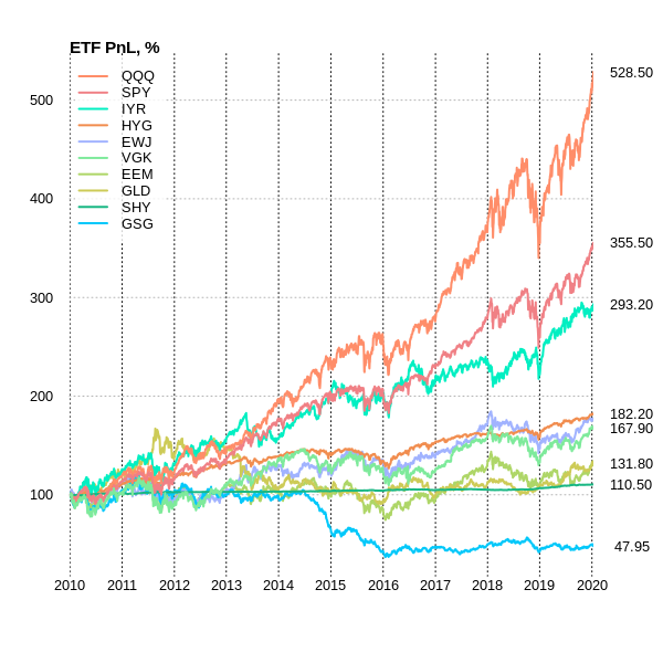
Today I will show how to apply the MC technique in a portfolio consisting of 10 ETFs using R and calculate Walk Forward statistics with monthly rebalance using a different set of evaluation metrics. So we have the following set of ETF:

Let’s see the ETF dynamic:

So now we will move to generate MC weights with certain restrictions: the weight of an ETF is non-negative and does not exceed 30%. The upper limit of 30% just in order to make the portfolio more diversified.

Also, we can have a look at the 1-step performance dynamic assuming in-sample period up to 2018–01–01 and out-of-sample after this date:

Here we can see how red points indicated efficient frontier on in-sample data performed on the out-of-sample period taking into all portfolio universe that satisfies the weight constraints.
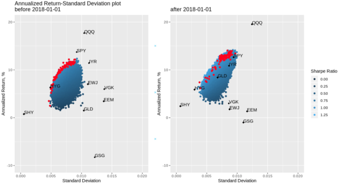
Now we will move to calculate walk forward tests maximizing the following metrics:
PnL;
PnL × R², (R-squared is the coefficient of determination);
PnL × R² / MaxDD;
Sharpe Ratio,
rolling on different intervals: 6, 12, 24, 36 months rebalancing monthly.
Using C++ functionality in R allows you to speed up your calculations. Rolling calculations on 10k different portfolios with 4 different intervals take seconds.
So here we got our unbiased performance using walk forward optimization:

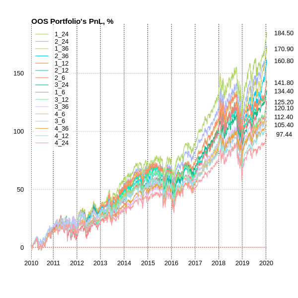
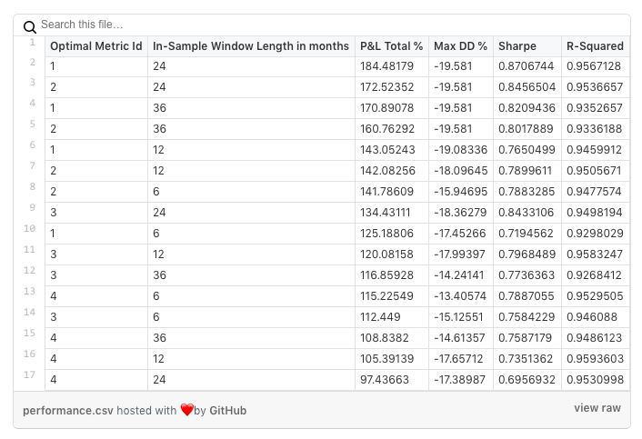
You can see that the best performance achieved applying PnL and PnL × R² optimization metrics with the In-Sample window equals 24 months.

This result also implies that from the point of view of productivity, the Sharpe Ratio optimization and small In-Sample windows (6 and 12 months) construct portfolios that by far the least productive.
Walk Forward Portfolio Optimization and the Monte Carlo method for generating asset weights shows the most accurate and unbiased performance results that an investor can get using certain risk and return preferences.
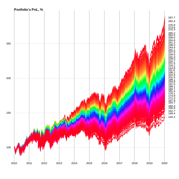
It also says that the result of choosing best portfolio generated by Monte Carlo simulation (presented in ‘ETF Portfolio Universe Dynamic’ chart) is not achievable and will give unsuccessful portfolio performance evaluations.
All code in order to replicate results can be found here.